Welcome to the website of Science Dynamics - a project of Proverbs, a.s.
")
")


System Dynamics
Whether a soft-phase in which a causal loop diagram (CLD) is created is necessary in system-dynamic projects is a matter of debate. After almost thirty years of experience, we consider the diagram to be a conditio sine qua non and do not work on projects without a diagram that expresses the underlying feedback structure and relationships.
If we have a diagram, we move to the System Dynamics field and the stage of converting the Causal Loop Diagram into a so-called Stock and Flow diagram (abbreviated as Flow diagram - FD) is ahead of us. In the article dedicated to CLD we wrote that they work with two types of elements - parameters and arrows (links).
Figure 1 Rules for converting a causal loop diagram to a flow diagram.
The purpose of system dynamics is to mathematize the CLD, to convert the diagram into a computer-simulable form, because mental simulation of a more complex CLD is not possible. However, two elements of a CLD are not enough to mathematically express the system structure. Four are needed. A flow, computer-simulable diagram requires the correct assignment of CLD elements to FD elements. The options are described in Figure 1.
The basic premise of System Dynamics is that dynamic behavior occurs when flows accumulate in levels. Thus, it can be said that if there is no accumulation of flows in levels, one cannot speak of dynamic behavior. The key element of any dynamic model is therefore the level (also called "stock" or "accumulation"). As stated in the previous paragraph, the purpose of System Dynamics is to mathematically express the system structure and to allow its simulation. The conversion of a CLD into a flow diagram must lead to the creation of at least one level. If we fail to do this, we are probably trying to model a static system. Each level must have at least one inflow or outflow.
The basic premise of System Dynamics is that dynamic behavior occurs when flows accumulate in levels. Thus, it can be said that if there is no accumulation of flows in levels, one cannot speak of dynamic behavior. The key element of any dynamic model is therefore the level (also called "stock" or "accumulation"). As stated in the previous paragraph, the purpose of System Dynamics is to mathematically express the system structure and to allow its simulation. The conversion of a CLD into a flow diagram must lead to the creation of at least one level. If we fail to do this, we are probably trying to model a static system. Each level must have at least one inflow or outflow.
The figure shows that the CDL parameter in the flow diagram changes to either a variable or a level. Furthermore, the CLD arrow becomes either a flow (inflow or outflow) or an information link in the flow diagram. The method of converting flow diagrams requires the knowledge you gain in our courses and literature. The procedure for creating a management simulator is described in the opening figure of this article. As with the CLD, we create the computer model so that it can answer the question with which we created the causal loop diagram. The management simulation project can be described in five steps:
1. The first step is to create a causal loop diagram using the System Thinking tools.
2. Run the appropriate software for creating system-dynamic models.
3. Convert the causal loop diagram into a flow diagram using specialized software (preferably Vensim).
4. We set up the finished computer model to simulate scenarios to find the answer to the question or questions posed.
5. We use the answers, verified by the simulation, to formulate management procedures that will lead to achieving the desired goals.
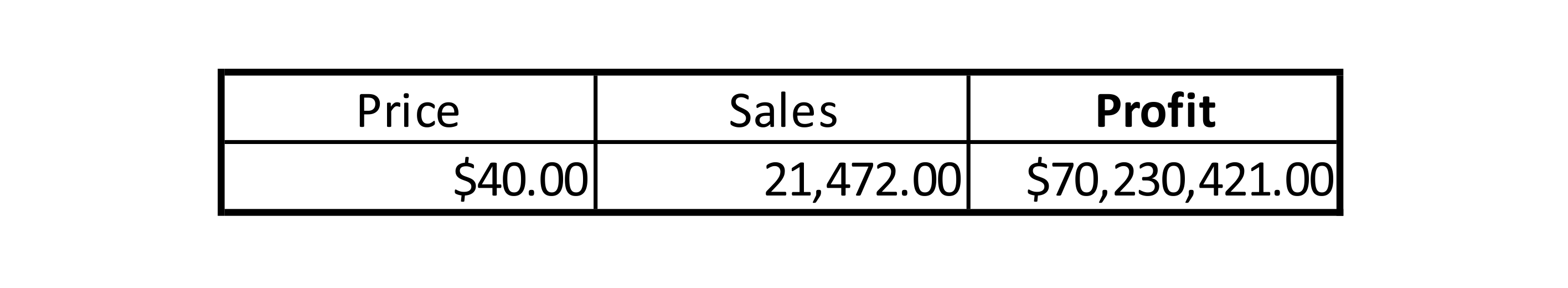
Figure 2 shows an example of a flow diagram (computer model) created in the Vensim simulation software. In creating the simulation model, the question "At what price will the profit be highest?" was addressed. You may be thinking that the highest profit will be at the highest price. Let's explore the validity of this statement together. In the following table, you will find a spreadsheet model that says that at a price of $40 per unit of product, 21,472 customers (1 customer - 1 unit of product purchased) will buy from us in week 60 and we will make a cumulative (gross) profit of $70,230,421. Just for completeness, the profit in week 60 is of course the product of the number of customers and the price of the product in the spreadsheet.
Unlike static spreadsheet models, the dynamic simulation model covers all the essential properties of real systems, namely:
a) Feedback
b) Delays
c) Non-linear variable relations
d) Complexity
Therefore, the simulation results of the dynamic model can be expected to differ significantly from those of the spreadsheet model, even though all input parameters are the same in both models. We will simulate the same period - 60 weeks with a time step of one week.
Figure 2 Flow diagram - simulation model - company structure created in simulation software.
Figure 3 Simulation results for the scenario at $40 per unit of product.
By simulating a scenario in which we set the price per unit of product to $40, we find that both the number of customers at the end of the period and the profit achieved are significantly lower than what the static spreadsheet model indicates. The simulation results can be seen in Figure 3. After sixty weeks, sales are at 3,355 units of product and profit achieved is $5,547,000. Assuming that one of the models is closer to reality, which one is it? The static model in the spreadsheet or the dynamic model in Vensim? Look at the structure of the flow diagram in Figure 2, specifically the effect of Price on model behavior. We find that Price is used to calculate Revenues. The calculation of Revenues is trivial in both models, Revenues = Price * Sales. In other words, the price per unit is multiplied by the number of units sold. What the dynamic model adds is the effect of Price on Demand. The dynamic model expresses the general fact that too high a price will lead to less interest in the product, and once a certain threshold is crossed, no one will be interested in the product anymore.
Does it make sense to introduce such rules into the model? If we really want to know how our business will behave, there is no doubt that it is worthwhile. What is the point of a model that tells us we will make a profit of 70 million when in reality it will be ten times less? So why don't we put the relationship between product price and demand into our static spreadsheet model? Because the relationship is non-linear and in static models we need to create a non-linear function in a separate spreadsheet that will affect the resulting demand value. The complexity of the solution is one of the reasons why in static models the non-linear relationships between variables are neglected and the results are then meaningless. In a dynamic model, a single variable is all that is needed to do this, in which the mouse is used to set up the course of the assumed relationship between price and its influence on demand (Influence of Price on Demand) as in Figure 4. In a few seconds, it is possible to set any relationship between variables and model soft variables that do not appear in static models, even though they play a key role in reality.
Figure 4 A simple way to set up a non-linear relationship between variables in a dynamic model.
Figure 5 Results of the simulation scenarios and product inventory detail.
But the problems with spreadsheets don't end there. Let's now look at the production part of our model. There is nothing to see in the spreadsheet. We have no idea how the elements of the model are connected, we have to examine each cell separately to see what affects its value. In the flow diagram, the logic of the model is expressed graphically. We can immediately see that current demand is used to calculate forecast demand and forecast demand determines the production. Production produces the products that go into the product warehouse and from there are shipped to the customer. Let us now set up our dynamic model again exactly according to the static model and look at the sales flow. The model works with two demand modes. Summer and year-round, called "stable". So far we have been working with the stable one. The sum is the same for both runs, only the distribution in the simulated period differs. The summer waveform is characterized by low demand in winter and high demand in summer. The summer demand waveform is reflected in Sales shown in Figure 4 by the red curve.
In terms of profit, the summer scenario is less successful, but take a look at the last chart, which shows Product stock. The red pattern shows that the inventories of the summer scenario are in negative values! So it means we are selling a product we don't have. How is this possible? Looking at the structure in Figure 2, we can see that the Sales value determines the outflow from the Product stock. Sales are only driven by demand, nothing else prevents them and the Stock value has no effect on Sales. In reality, however, it does not work this way. If we are selling a physical product, we need to actually deliver it to the customer, otherwise we run the risk of prosecution for fraud. Is there any solution to the problem of selling non-existent products? Very easily in the dynamic model. We simply add the feedback from the stock of products to the definition of Sales and say that Sales cannot be higher than the Stock of finished products as in Figure 6. In the output graphs we see that even in the summer scenario the stock does not fall below zero and the feedback therefore works! In Figure 2, the feedback from Product stock to Sales is highlighted with a red color. Can the problem be solved in a spreadsheet as well? The answer may surprise you - it cannot. The spreadsheet displays an error message when you try to create a feedback loop, stating that you are trying to create an illegal circular dependency. The problem is that the nature of all systems in this world is based on circular dependencies! So this means that real world models cannot be created in a spreadsheet.
Figure 6 Simulation of scenarios with feedback that prevents the sale of non-existent products.
Figure 7 Results of the simulation scenarios after delays are introduced.
However, the problems with static models in spreadsheets do not end there. Anyone who works in the real world knows that there is often a very significant delay between action and reaction. In our simple business, for example, there is a delay between the time products are entered into production and placed in the warehouse, and between the order and delivery to the customer. But there is an even more significant delay between the investment in marketing and its effect on demand. The delay is variable, depending on the scale of the marketing campaign. In system diagrams, the delay is usually indicated by two perpendicular lines on an arrow, as in Figure 2 between Influence of marketing on demand and Demand. In our dynamic model, we plug in the not-yet-applied marketing and, more importantly, we introduce a production delay of 3 weeks and a product shipment delay of 2 weeks, exactly as in the actual firm we are modeling. In the spreadsheet models, no delays can be captured and so the results are calculated as if the delays do not exist. The results in Figure 7 show that the delay actually implies a lower inventory volume. Imagine that you are making a plan for the next year and in it you calculate the capital required, which will be 100% higher than in reality. And we haven't yet put in delays in material supply, human resources, accounts payable, accounts receivable, and potential claims. But it is already clear that the spreadsheet's ability to capture the real behavior of the business is marginal compared to the dynamic model.
If you have read this far, it means that you are interested in the topic and, more importantly, you are eager to learn. We welcome you to our training programs, we will teach you everything you need to build models capable of capturing the real-world behavior of businesses, public policy, and indeed anything that changes over time. Don't forget to check out our software and literature.